Neural Networks: Forward Propagation

We will describe the usage of neural networks for multiclass classification. A concrete example is the recognition of hand-written digits 0, 1, 2, ...9. A possible approach is as follows:
The images of the digits are normalized into say 20x20 pixel images of gray values from 0-255. One pixel corresponds to a "feature", so there are 400 input features. The output of the networks is one of the 10 classes '0', '1', '2', ...'9'. The figure below shows a possible neural network.

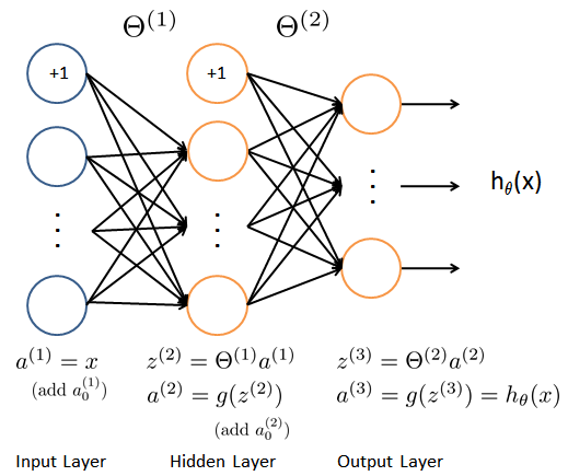
The input layer has 400 neurons corresponding to the image features, plus a bias unit that has always the value '1'. Then, there is one hidden layer with say 25 neurons plus a bias unit. Finally, there is an output layer with 10 neurons corresponding to the 10 classes: the neuron 1 corresponds to the digit '1', the neuron 2 corresponds to the digit '2', etc., and the neuron 10 corresponds to the digit '0'. If e.g. the class '3' was recognized, then the output should be ideally (0, 0, 1, 0, ... 0)^T. (T denotes the transpose.) In practice, it will be $h = (h_1, h_2, ... h_{10})^T$ where $h_i$ is the probability that the input belongs to the class $i$. We would then choose that class $i$ whose $h_i$ is the maximum ($h_3$ in our example).

To compute the prediction $h$, the vector $x = (x_1, ... x_N)^T$ of input features (N = 400) is propagated through the network. We assume that the network has L levels and $N_l$ neurons at the level $l$ not counting the bias neurons.

$N_1 = N$ (number of features)

$N_L = K$ (number of classes)

We define the "activations" (values of the neurons) at the input level as the input features $a^{(1)} = (x_1, ... x_N)^T$.

At each level $l, l = 2, 3, ...L$ we compute the activations from the previous level:

$$ z^{(l)} = \Theta^{(l-1)} a^{(l-1)} \; \text{, i.e. matrix} \times \text{vector} $$

$$ a^{(l)} = [1; g(z^{(l)})] = \left[ \begin{array}{c} 1 \\ g(z_1^{(l)}) \\ \dots \\ g(z_{N_l}^{(l)}) \end{array} \right] $$

We used the MATLAB/Octave notation $[1; v]$ to denote the column vector with first element "1" and the other elements equal to the elements of $v$. The dimension of this compound vector is $1 + \dim(v)$. At the last level L we do not extend the vector $a$ by "1", so $a^{(L)} = g(z^{(L)})$.

g(z) is the sigmoid function

$g(z) = \frac{1}{1 + e^{-z}}$

that is applied to each element of the vector z.

Finally, at the last level L, we get the prediction vector:

$h_\Theta(z) = a^{(L)}$

The matrix $\Theta^{(l)}, l = 1, 2, ..., L-1$ describes the transition from the level $l$ to the level $l+1$. It has the form:

$$ \Theta^{(l)} = \left[ \begin{array}{cccc} \Theta_{10}^{(l)} & \Theta_{11}^{(l)} & \dots & \Theta_{1N_l}^{(l)} \\ \Theta_{20}^{(l)} & \Theta_{21}^{(l)} & \dots & \Theta_{2N_l}^{(l)} \\ \dots & \dots & \dots & \dots \\ \Theta_{N_{l+1}0}^{(l)} & \Theta_{N_{l+1}1}^{(l)} & \dots & \Theta_{N_{l+1}N_l}^{(l)} \\ \end{array} \right] $$

and the dimension $\dim(\Theta^{(l)}) = N_{l+1} \times (N_l + 1)$. Notice further that:

$$ \begin{align} \dim(\Theta^{(l-1)}) & = N_{l} \times (N_{l-1} + 1) \\ \dim(a^{(l-1)}) & = N_{l-1} + 1 \\ \dim(z^{(l)}) & = N_l \\ \dim(a^{(l)}) & = N_l + 1 \\ \end{align} $$

Content